Introductory Tutorials#
This section provides an overview of the basic functionalities offered by CRISP. Each tutorial introduces a specific feature of the package, guiding you through typical use cases.
First verify the installation by importing CRISP and its dependencies:
import CRISP
print(f"CRISP version: {CRISP.__version__}")
CRISP is organized into two main subpackages:
simulation_utility: Tools for preparing and processing simulation datadata_analysis: Methods for analyzing simulation results
The following tutorials are organized according to these subpackages.
Simulation Utility#
This section covers utilities for manipulating and preparing simulation data.
Atomic Indices#
CRISP allows for the classification of atoms based on custom-defined indices, making it easier to analyze specific subsets within your simulation data.
Classify Atom Indices
from CRISP.simulation_utility.atomic_indices import run_atom_indices # Path to your ASE trajectory file file_path = "./wrapped_traj.traj" # Output folder to save the indices output_folder = './indices_new/' # Define the custom cutoffs dictionary custom_cutoffs = { ("O", "H"): 1.2, ("Si", "O"): 1.8, ("Al", "Si"): 3.2, ("O", "O"): 3.0 } # Run the atom_indices function and save the results with a specific frame index run_atom_indices(file_path, output_folder, frame_index=10, custom_cutoffs=custom_cutoffs)
Output:
Analyzing frame with index 10 (out of 21 frames) Length of O indices: 432 Length of H indices: 120 Length of Si indices: 168 Length of Al indices: 24 Outputs saved. Saved cutoff indices for O-H to ./indices_new/cutoff/O-H_cutoff.csv Saved cutoff indices for Si-O to ./indices_new/cutoff/Si-O_cutoff.csv Saved cutoff indices for Al-Si to ./indices_new/cutoff/Al-Si_cutoff.csv Saved cutoff indices for O-O to ./indices_new/cutoff/O-O_cutoff.csv
Atomic Trajectory Visualization#
Visualize atomic trajectories in 3D to understand motion and structural changes.
from CRISP.simulation_utility.atomic_traj_linemap import plot_atomic_trajectory
# Path to trajectory file
traj_file = "./wrapped_traj.traj"
# Output directory for the visualization
output_dir = "./atomic_traj_linemap/o593_atom_trajectory.html"
# Select specific atom for trajectory analysis
selected_atoms = [593]
# Generate interactive 3D visualization of trajectories
fig = plot_atomic_trajectory(
traj_path=traj_file,
indices_path=selected_atoms,
output_dir=output_dir,
frame_skip=1,
plot_title="Oxygen Atom Movement Analysis",
atom_size_scale=1.2,
show_plot=True
)
Output:
Loading trajectory from ./wrapped_traj.traj (using every 1th frame)...
Loaded 21 frames from trajectory
Using 1 directly provided atom indices for trajectory plotting
Simulation box dimensions: [24.34499931 24.34499931 24.34499931] Å
Analyzing atom types in first frame (total atoms: 744, max index: 743)...
Found 4 atom types: Si, Al, O, H
Plot has been saved to ./atomic_traj_linemap/o593_atom_trajectory.html/trajectory_plot.html
Visualisation Output:
This interactive 3D visualization allows you to:
Rotate, zoom, and pan to explore atomic trajectories
Track the movement of selected atoms over time
Visualize the trajectory path with customizable atom sizes
Understand atomic motion patterns within the simulation box
Subsampling#
Extract representative structures from a trajectory using Farthest Point Sampling.
from CRISP.simulation_utility.subsampling import subsample
# Extract representative structures from trajectory
all_frames = subsample(
traj_path="./wrapped_traj.traj",
n_samples=10,
index_type="all",
file_format="traj",
frame_skip=1,
plot_subsample=True,
output_dir="./Subsmapling"
)
print(f"Selected {len(all_frames)} representative structures")
Output:
Saved convergence plot to ./Subsmapling/subsampled_convergence.png
Saved 10 subsampled structures to ./Subsmapling/subsample_wrapped_traj.traj
Visualisation Output:
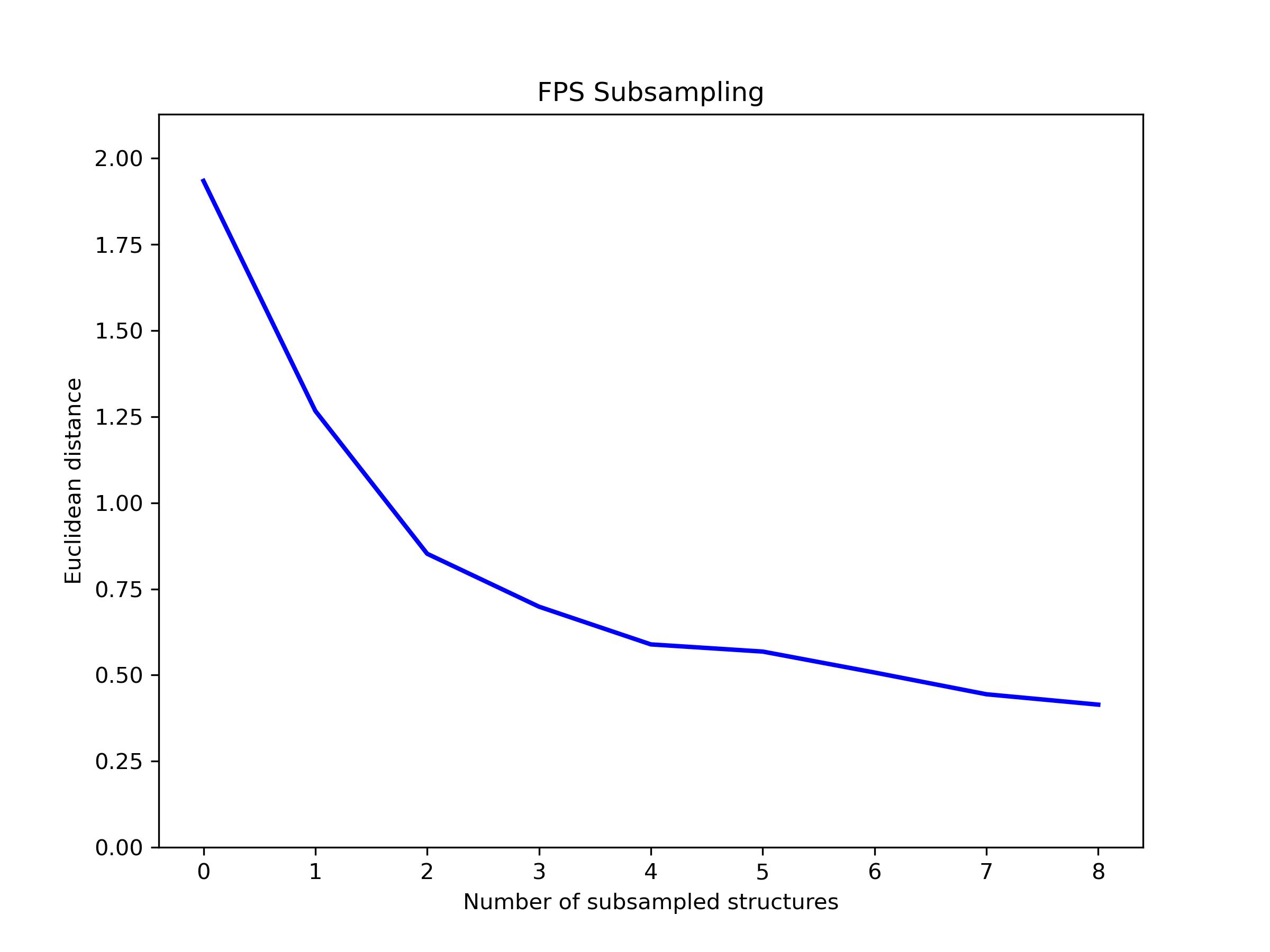
The convergence plot shows the distance between each sampled structure and its nearest neighbor, illustrating how the algorithm selects maximally diverse structures from the trajectory.
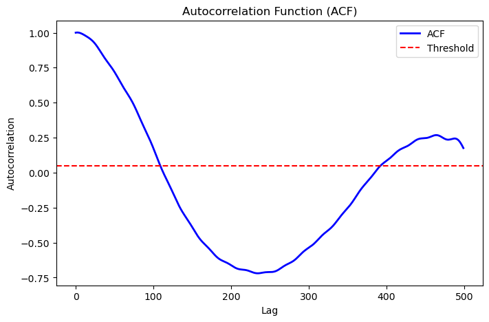
Error Analysis#
Perform statistical error analysis on time-correlated simulation data using different methods.
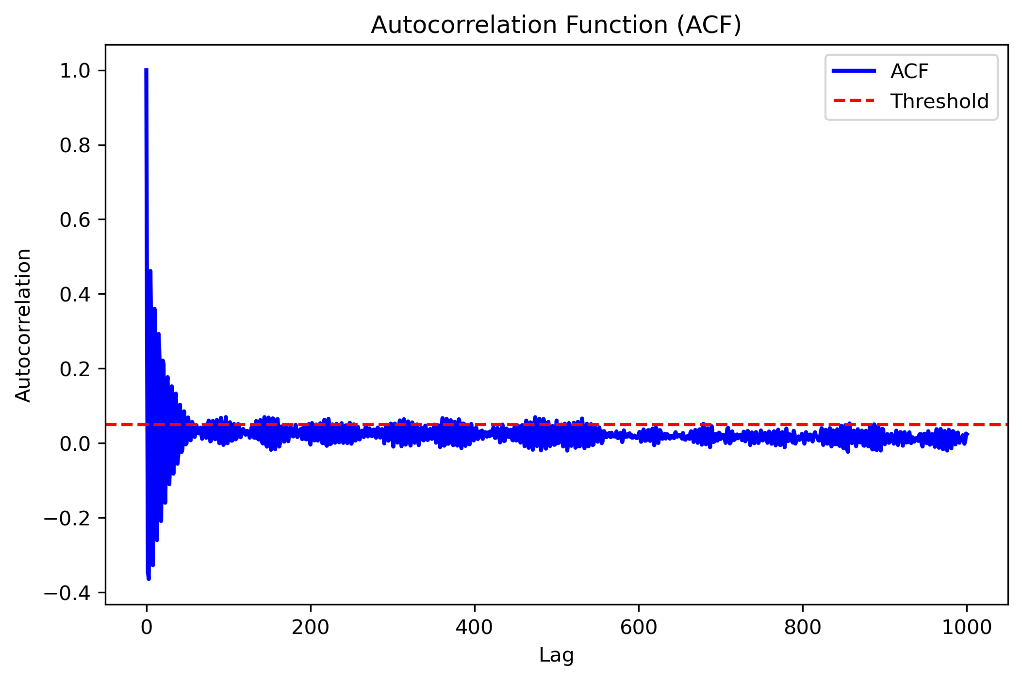
Example 1: Position Data Analysis#
from CRISP.simulation_utility.error_analysis import autocorrelation_analysis
import numpy as np
# Load position data
data_positions = np.load("./error/positions.npy")
# Analyze using autocorrelation method
res_positions = autocorrelation_analysis(
data_positions,
plot_acf=True,
max_lag=500
)
print(res_positions)
Output:
{'mean': array([11.84336219, 6.56230374, 6.34512439]),
'acf_err': array([0.11042688, 0.0483816 , 0.06882431]),
'std': array([0.21002227, 0.09201757, 0.13089782]),
'tau_int': 69.11286151958006,
'optimal_lag': 109}
Visualization Output:
Example 2: Energy Data Analysis#
from CRISP.simulation_utility.error_analysis import autocorrelation_analysis, block_analysis
import numpy as np
# Load energy data from log file
data_energy = np.loadtxt("./error/md_20k.log", skiprows=1, usecols=2)
# Analyze using autocorrelation method
acf_error = autocorrelation_analysis(data_energy, plot_acf=True)
# Analyze using blocking method
block_error = block_analysis(data_energy, convergence_tol=0.001, plot_blocks=False)
print(acf_error)
print(block_error)
Output:
{'mean': -3065.5796212000005,
'acf_err': 0.0054549762052233325,
'std': 0.6834300195116669,
'tau_int': 0.318542675191111,
'optimal_lag': 9}
{'mean': -3065.5796212000005,
'block_err': 0.02208793396091249,
'std': 0.6834300195116669,
'converged_blocks': 32}
Visualization Output:
Interatomic Distance Calculation#
Calculate and save distance matrices between atoms for further analysis.
from CRISP.simulation_utility.interatomic_distances import distance_calculation, save_distance_matrices
# Path to trajectory file
traj_path = "./wrapped_traj.traj"
frame_skip = 10
index_type = ["O"] # Focus on oxygen atoms
# Calculate full and subset distance matrices
full_dms, sub_dms = distance_calculation(traj_path, frame_skip, index_type)
# Save the calculated distance matrices
save_distance_matrices(full_dms, sub_dms, index_type, output_dir="distance_calculations_zeo")
Output:
Distance matrices saved in 'distance_calculations_zeo/distance_matrices.pkl'
This utility calculates distance matrices between atoms, accounting for periodic boundary conditions, and saves the results for later use in clustering or other analyses.
Data Analysis#
This section covers methods for analyzing simulation results and extracting physical insights.
Contact and Coordination Analysis#
CRISP provides tools to analyze both coordination environments and dynamic contacts between atoms.
1. Coordination Analysis#
from CRISP.data_analysis.contact_coordination import coordination
# Path to trajectory file
filename = "./wrapped_traj.traj"
# Define target and bonded atoms for coordination analysis
target_atoms = "O"
bonded_atoms = ["O"]
# Define custom cutoffs for coordination
custom_cutoffs = {('Al', 'O'): 3.5, ('O', 'O'): 2.5}
# Perform coordination analysis
cn = coordination(filename,
target_atoms, bonded_atoms, custom_cutoffs,
skip_frames=10, plot_cn=True, output_dir="./CN_data")
Output:
Interactive coordination distribution chart saved to ./CN_data/CN_distribution.html
Visualization Output:
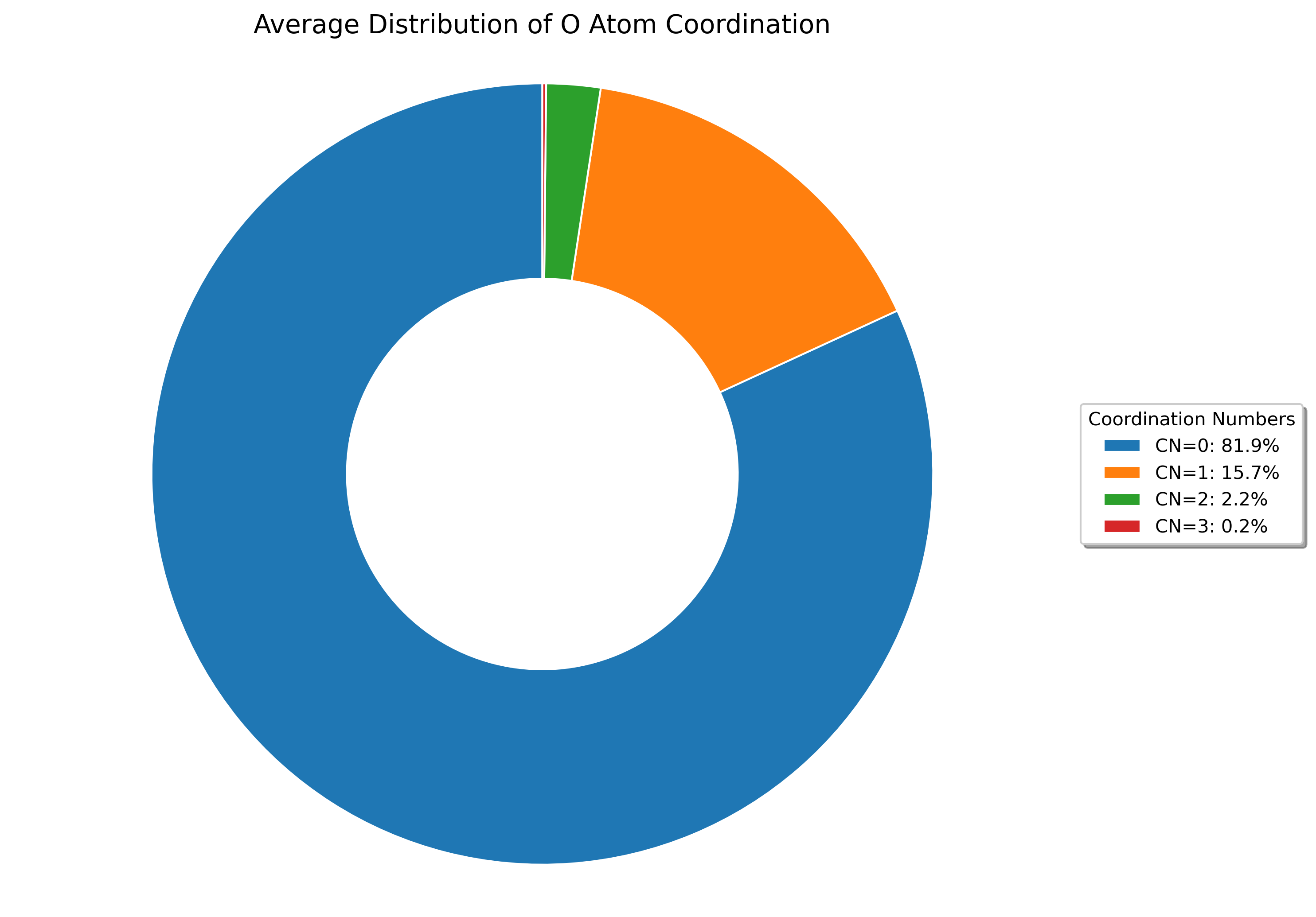
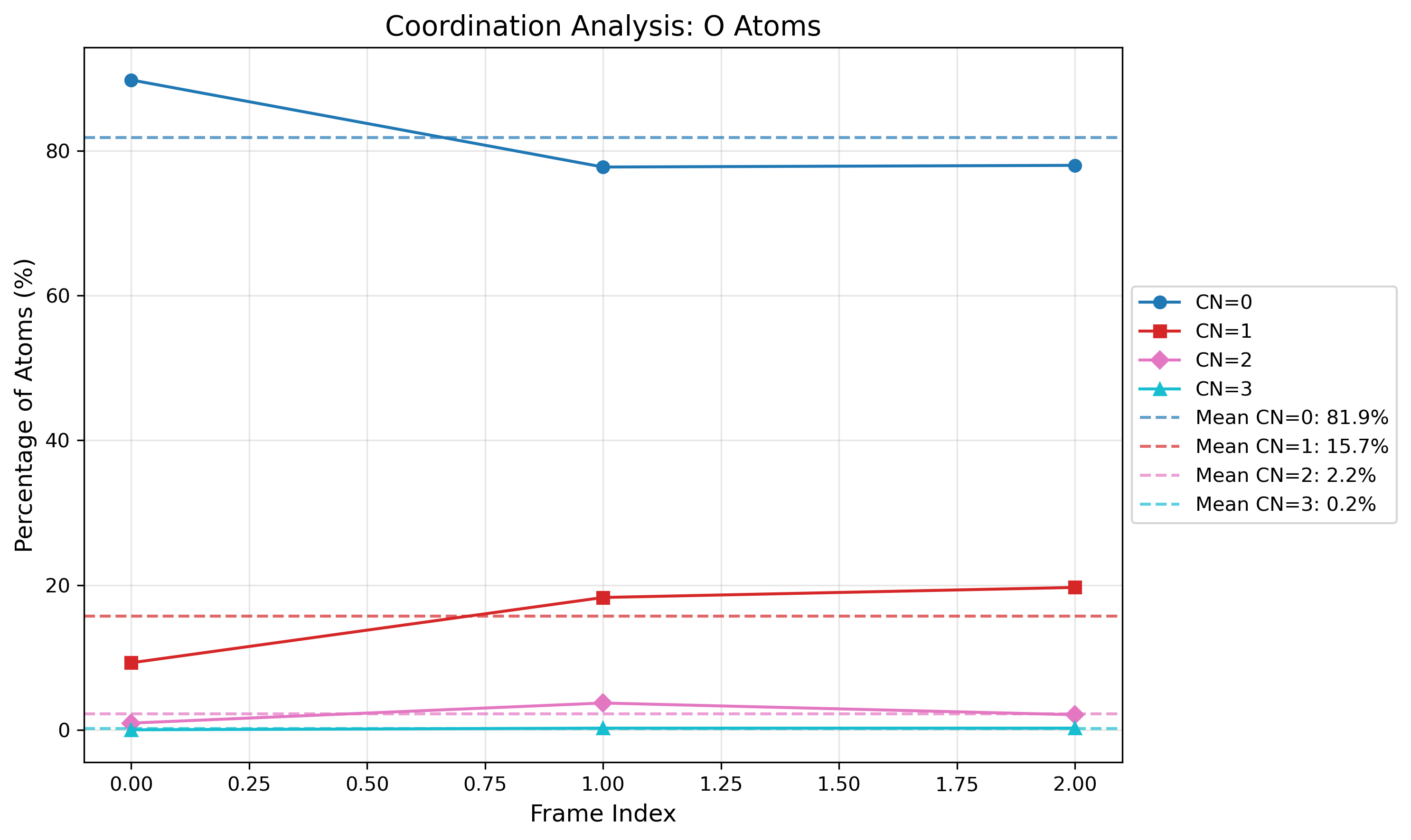
The visualizations show both: - The distribution of coordination numbers across all analyzed frames, revealing dominant coordination environments - The time evolution of coordination numbers throughout the trajectory, showing structural changes over time
The visualization shows the distribution of coordination numbers for the selected atom types, allowing you to identify dominant coordination environments and their frequencies throughout the simulation trajectory.
2. Contact Analysis#
from CRISP.data_analysis.contact_coordination import contacts
# Path to trajectory file
filename = "./wrapped_traj.traj"
# Define target and bonded atoms for contact analysis
target_atoms = "O"
bonded_atoms = ["O"]
# Define custom cutoffs for contacts
custom_cutoffs = {('Al', 'O'): 3.5, ('O', 'O'): 2.5}
# Perform contact analysis
sub_dm, cal_contacts = contacts(
filename, target_atoms, bonded_atoms, custom_cutoffs,
skip_frames=1,
plot_distance_matrix=True,
plot_contacts=True,
time_step=50.0*1000, # fs
output_dir="./Contacts_data")
Output:
Interactive contact heatmap saved to ./Contacts_data/O_heatmap_contacts.html
Interactive contact analysis chart saved to ./Contacts_data/average_contact_analysis.html
Static contact analysis chart saved to ./Contacts_data/average_contact_analysis.png
Interactive distance heatmap saved to ./Contacts_data/O_heatmap_distance.html
Visualization Output:
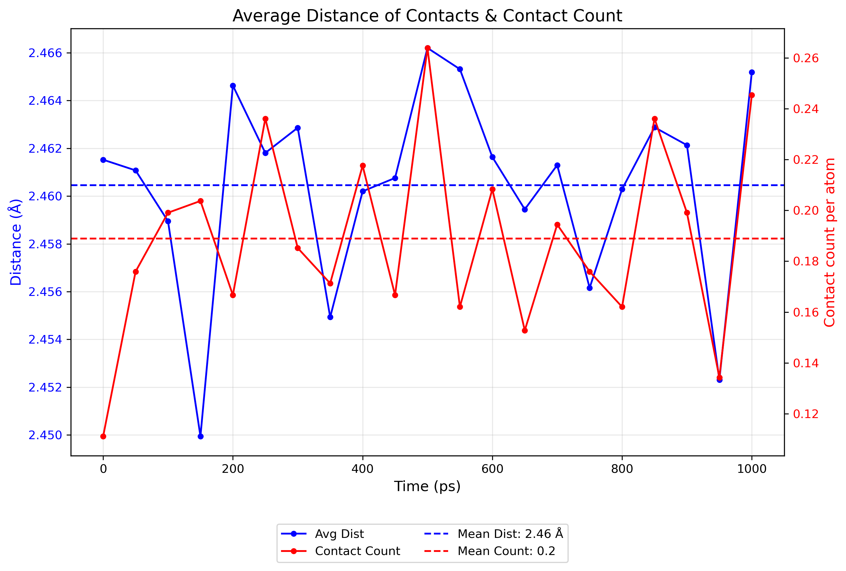
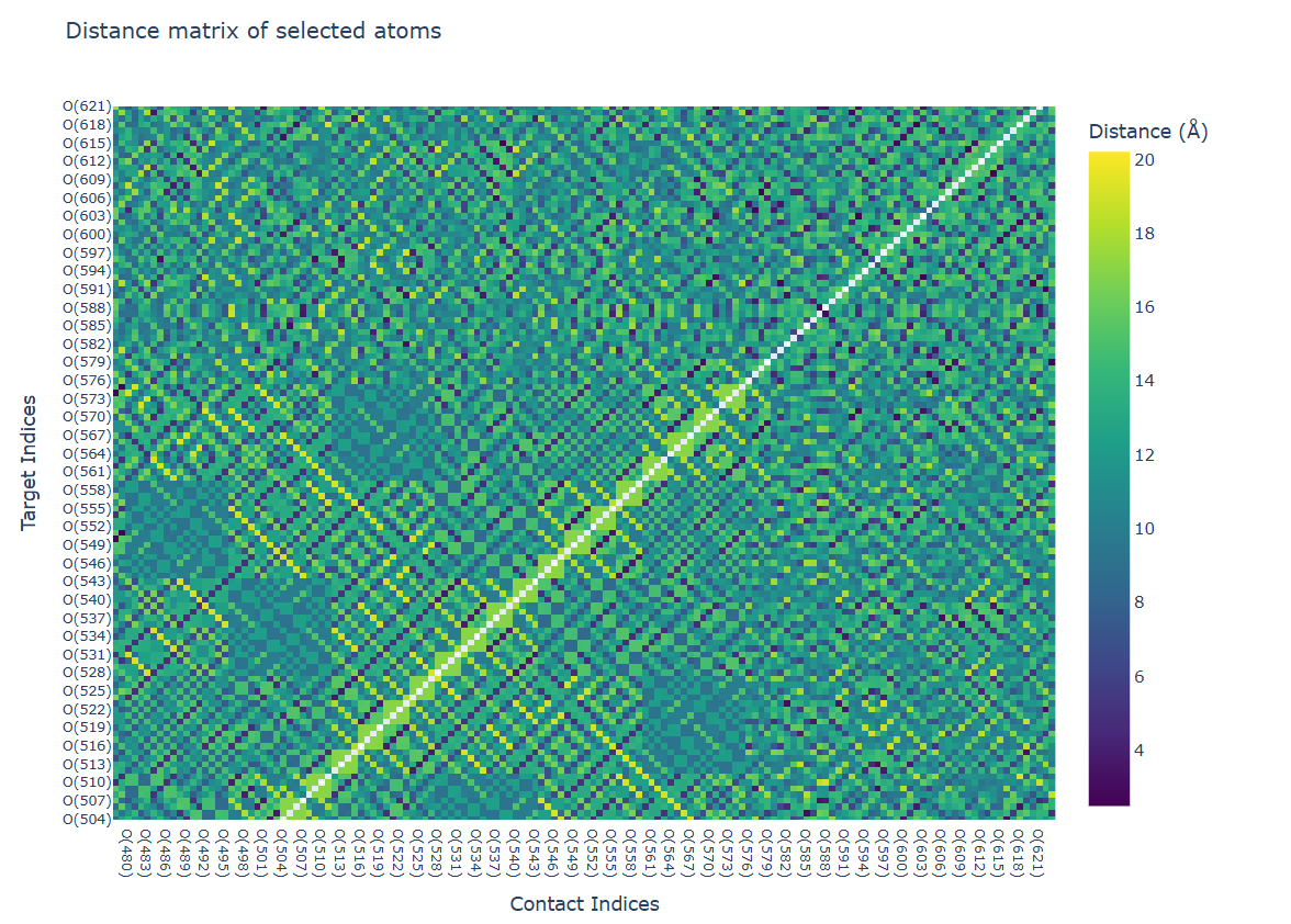
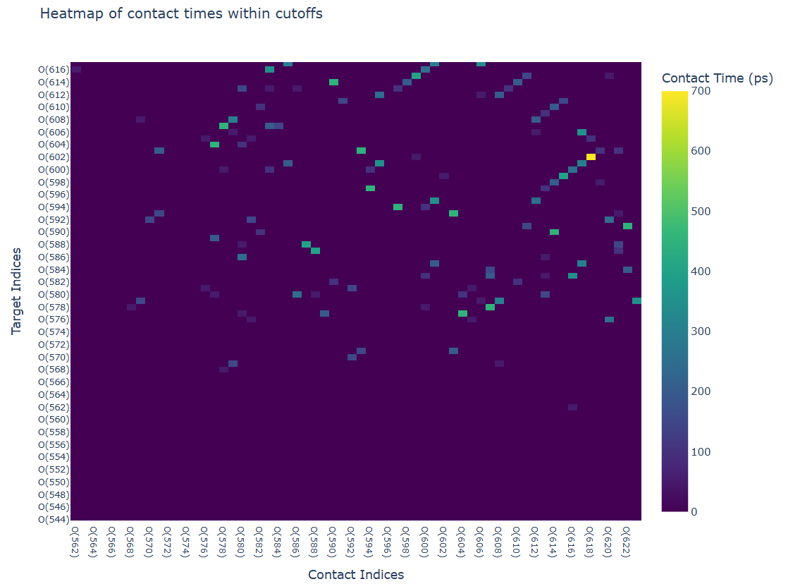
- The contact analysis provides multiple visualizations:
A summary of average contact statistics and their distribution
A distance heatmap showing the spatial relationships between atoms
A time heatmap showing the persistence of contacts throughout the trajectory
These visualizations enable the identification of persistent contacts and transient interactions throughout the simulation trajectory.
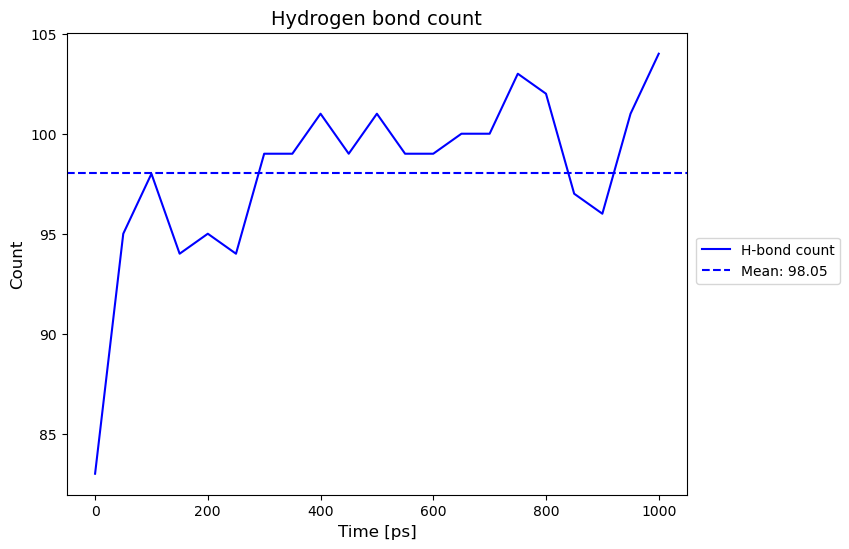
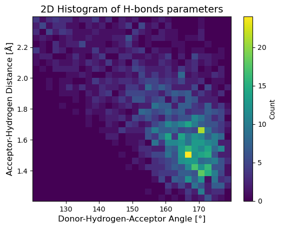
Hydrogen-Bonding Analysis#
Analyze hydrogen bond networks and dynamics in your simulation.
from CRISP.data_analysis.h_bond import hydrogen_bonds
# Perform hydrogen bond analysis
h_bonds_both_plots = hydrogen_bonds(
traj_path="./wrapped_traj.traj",
frame_skip=1,
acceptor_atoms=["O"],
angle_cutoff=120,
mic=True,
output_dir="./H_Bond_Data",
time_step=50*1000,
plot_count=True,
plot_heatmap=True,
plot_graph_frame=True, # Generate frame-specific plot
plot_graph_average=True, # Generate average plot
graph_frame_index=10 # Use frame 10 instead of default 0
)
Output:
Hydrogen bond count plot saved to './H_Bond_Data/h_bond_count.png'
H-bond structure 2D histogram saved to './H_Bond_Data/h_bond_structure.png'
Generated and saved 196 unique donor/acceptor atom indices to ./H_Bond_Data/donor_acceptor_indices.npy
Generating hydrogen bond network visualizations for frame 10...
Interactive correlation matrix saved as './H_Bond_Data/hbond_correlation_matrix_frame_10.html'
Figure saved as './H_Bond_Data/hbond_network_frame_10.html'
Generating average hydrogen bond network visualization...
Interactive correlation matrix saved as './H_Bond_Data/hbond_correlation_matrix_average.html'
Figure saved as './H_Bond_Data/hbond_network_average.html'
Visualization Output: